Fitting Multiple Sources in an Image

In this walkthrough, we will show the extension of pysersic from a single source to an image with multiple sources. Let’s get started with our imports, and loading up one of the example galaxies.

[1]:

from pysersic import FitMulti, PySersicMultiPrior
from pysersic.results import parse_multi_results
from pysersic.loss import *
import numpy as np
import matplotlib.pyplot as plt

import arviz as az
import sep
from jax.random import PRNGKey
import copy

num = 3
im = np.load(f'./examp_gals/gal{num:d}_im.npy')
mask = np.load(f'./examp_gals/gal{num:d}_mask.npy')
psf = np.load(f'./examp_gals/gal{num:d}_psf.npy')
rms = np.load(f'./examp_gals/gal{num:d}_sig.npy')
plt.imshow(np.log10(im));

/var/folders/55/yk32fyfs7kzf9l80rvr6bmg40000gn/T/ipykernel_76843/776769578.py:17: RuntimeWarning: invalid value encountered in log10
  plt.imshow(np.log10(im));

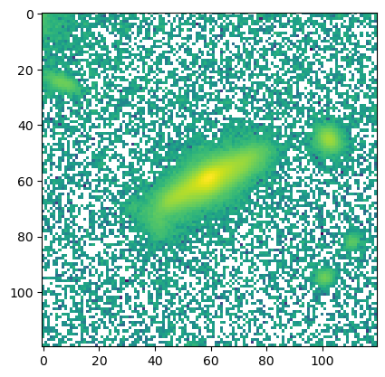
As we can see, this image has ~5 galaxies of different sizes and shapes. If we were only interested in the central, we could mask the rest. But we can also jointly fit them all.

To begin, we need to construct a catalog of sources, with prior guesses for the positions and sizes of each. You can construct catalogs however you like (e.g., from source extractor); here, we’ll use the sep package to quickly find these sources and catalog them.

[2]:

#Simple Source Finder to generate catalog
objs,smap = sep.extract(im, 5, err = rms, segmentation_map = True,  deblend_cont=5e-5)
to_pysersic = {}
to_pysersic['flux'] = objs['flux']
to_pysersic['x'] = objs['x']
to_pysersic['y'] = objs['y']
to_pysersic['r'] = objs['a']

type_list = []
for j in range(len(to_pysersic['x'])):
    if to_pysersic['flux'][j] < 30:
        type_list.append('pointsource')
    else:
        type_list.append('sersic')
to_pysersic['type'] = type_list
to_pysersic

[2]:

{'flux': array([  36.08848572,   83.98748016, 1476.61169434,   10.08358097,
          16.07361984]),
 'x': array([  6.67035738, 102.28865071,  58.83336503, 110.93241678,
        100.73941897]),
 'y': array([25.00044378, 45.36315877, 60.08400813, 81.94876027, 94.75703145]),
 'r': array([3.44829583, 2.63860273, 9.26280499, 1.66357291, 1.72083819]),
 'type': ['sersic', 'sersic', 'sersic', 'pointsource', 'pointsource']}

As we can see, the format of the catalog is a dictionary (or dataframe) with keys flux, x, y, r, and type. The type designation is used to specify the type of fit to perform; for point sources, you can choose the point source option.

Armed with a catalog, we can now create a PySersicMultiPrior object.

If you are setting the sky_type to None (that is, not fitting for any sky background), you can proceed with creating the prior. If you are fitting the sky, we need to create an estimate for the sky level and rms.

This can be easily done with the priors.estimate_sky function.. We’ll make a masked version of our input image to mask everything but the central source, so that we can use pixels around the border to make an estimate of the sky.

[3]:

from pysersic.priors import estimate_sky
med_sky, std_sky, n_pix = estimate_sky(im, mask)
sky_guess = med_sky
sky_guess_err = 2.* std_sky / np.sqrt(n_pix) # Use twice the error on the mean as the prior width
print(sky_guess)
print(sky_guess_err)

0.01438230648636818
0.002397728894039896

Now that we have our sky estimates, we can create our prior from the catalog, specifying how to fit the sky:

[4]:

mp = PySersicMultiPrior(catalog = to_pysersic, sky_type='flat',sky_guess=sky_guess,sky_guess_err=sky_guess_err)
print (mp)

PySersicMultiPrior containing 5 sources
Source #0 of type - sersic:
---------------------------
xc_0 ---  Normal w/ mu = 6.67, sigma = 1.00
yc_0 ---  Normal w/ mu = 25.00, sigma = 1.00
flux_0 ---  Normal w/ mu = 36.09, sigma = 12.01
r_eff_0 ---  Truncated Normal w/ mu = 3.45, sigma = 3.71, between: 0.50 -> inf
n_0 ---  Uniform between: 0.65 -> 8.00
ellip_0 ---  Uniform between: 0.00 -> 0.90
theta_0 ---  Uniform between: 0.00 -> 6.28
Source #1 of type - sersic:
---------------------------
xc_1 ---  Normal w/ mu = 102.29, sigma = 1.00
yc_1 ---  Normal w/ mu = 45.36, sigma = 1.00
flux_1 ---  Normal w/ mu = 83.99, sigma = 18.33
r_eff_1 ---  Truncated Normal w/ mu = 2.64, sigma = 3.25, between: 0.50 -> inf
n_1 ---  Uniform between: 0.65 -> 8.00
ellip_1 ---  Uniform between: 0.00 -> 0.90
theta_1 ---  Uniform between: 0.00 -> 6.28
Source #2 of type - sersic:
---------------------------
xc_2 ---  Normal w/ mu = 58.83, sigma = 1.00
yc_2 ---  Normal w/ mu = 60.08, sigma = 1.00
flux_2 ---  Normal w/ mu = 1476.61, sigma = 76.85
r_eff_2 ---  Truncated Normal w/ mu = 9.26, sigma = 6.09, between: 0.50 -> inf
n_2 ---  Uniform between: 0.65 -> 8.00
ellip_2 ---  Uniform between: 0.00 -> 0.90
theta_2 ---  Uniform between: 0.00 -> 6.28
Source #3 of type - pointsource:
--------------------------------
xc_3 ---  Normal w/ mu = 110.93, sigma = 1.00
yc_3 ---  Normal w/ mu = 81.95, sigma = 1.00
flux_3 ---  Normal w/ mu = 10.08, sigma = 6.35
Source #4 of type - pointsource:
--------------------------------
xc_4 ---  Normal w/ mu = 100.74, sigma = 1.00
yc_4 ---  Normal w/ mu = 94.76, sigma = 1.00
flux_4 ---  Normal w/ mu = 16.07, sigma = 8.02
sky type - flat
sky_back --- Normal with mu = 1.438e-02 and sd = 2.398e-03

As we can see, we’ve now set up priors for each source in our image, as well as the sky. Unlike for the single source (where we can auto-guess these), the values are coming from the catalog file, under the assumption that flux, x,y, and r effective are measured (at least roughly).

Armed with our prior, we can now create a FitMulti object and decide how we are going to proceed with fitting. In this first example, we’ll simply find the MAP value, using a gaussian_mixture loss function and the HybridRenderer.

[5]:

fm = FitMulti(data = im, rms= rms, psf = psf, prior= mp)
map_dict = fm.find_MAP(rkey = PRNGKey(99))

 14%|█▍        | 2830/20000 [00:15<01:34, 180.80it/s, Round = 0,step_size = 5.0e-02 loss: -5.828e+03]
  1%|▏         | 254/20000 [00:01<01:27, 225.55it/s, Round = 1,step_size = 5.0e-03 loss: -5.827e+03]
  1%|▏         | 254/20000 [00:01<01:20, 246.76it/s, Round = 2,step_size = 5.0e-04 loss: -5.827e+03]

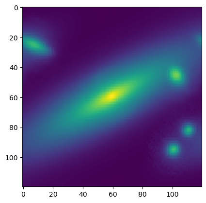
We can examine the MAP model:

[6]:

plt.imshow(np.log10(map_dict['model']));

As well as the residual between this model and the data, scaled by the rms:

[7]:

plt.imshow((map_dict['model']-im)/rms,vmin=-40,vmax=40,cmap='seismic')
plt.colorbar()

[7]:

<matplotlib.colorbar.Colorbar at 0x2cc6307f0>

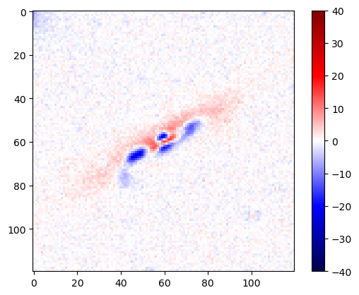
While most of the sources (besides the central one) are well fit, there’s clearly a lot of residual structure for the central source. In this case, these likely represent true deviations from a simple, smooth Sersic profile; in the raw imaging, we can see bulge like structure, for example.

As for single sources, we can go beyond a MAP estimate and use SVI to estimate the posterior space:

[8]:

fm.estimate_posterior(method = 'laplace', rkey = PRNGKey(999))
res_mp = fm.svi_results
res_mp.summary()

  6%|▋         | 1273/20000 [00:04<01:11, 261.64it/s, Round = 0,step_size = 5.0e-02 loss: -5.805e+03]
  1%|▏         | 262/20000 [00:00<01:15, 262.85it/s, Round = 1,step_size = 5.0e-03 loss: -5.805e+03]
  1%|▏         | 256/20000 [00:01<01:18, 252.90it/s, Round = 2,step_size = 5.0e-04 loss: -5.805e+03]
arviz - WARNING - Shape validation failed: input_shape: (1, 1000), minimum_shape: (chains=2, draws=4)

[8]:

	mean	sd	hdi_3%	hdi_97%	mcse_mean	mcse_sd	ess_bulk	ess_tail	r_hat
ellip_0	0.809	0.022	0.769	0.848	0.001	0.001	783.0	757.0	NaN
ellip_1	0.393	0.017	0.362	0.426	0.001	0.000	1055.0	868.0	NaN
ellip_2	0.763	0.001	0.762	0.764	0.000	0.000	922.0	841.0	NaN
flux_0	38.439	1.525	35.640	41.352	0.052	0.037	849.0	817.0	NaN
flux_1	79.685	2.144	76.001	83.721	0.066	0.047	1066.0	930.0	NaN
flux_2	1638.745	3.066	1632.576	1643.946	0.103	0.073	894.0	1026.0	NaN
flux_3	10.157	0.293	9.630	10.692	0.010	0.007	939.0	800.0	NaN
flux_4	15.672	0.275	15.194	16.236	0.009	0.007	862.0	923.0	NaN
n_0	0.731	0.082	0.655	0.873	0.003	0.002	914.0	881.0	NaN
n_1	0.814	0.059	0.714	0.923	0.002	0.001	1086.0	986.0	NaN
n_2	2.278	0.010	2.259	2.297	0.000	0.000	966.0	857.0	NaN
r_eff_0	4.011	0.148	3.727	4.293	0.005	0.003	1000.0	821.0	NaN
r_eff_1	2.085	0.041	2.009	2.163	0.001	0.001	965.0	982.0	NaN
r_eff_2	9.603	0.029	9.546	9.653	0.001	0.001	938.0	959.0	NaN
sky_back	0.002	0.000	0.001	0.003	0.000	0.000	752.0	868.0	NaN
theta_0	0.429	0.015	0.401	0.456	0.001	0.000	789.0	915.0	NaN
theta_1	0.923	0.025	0.878	0.969	0.001	0.001	826.0	944.0	NaN
theta_2	2.641	0.001	2.640	2.642	0.000	0.000	986.0	937.0	NaN
xc_0	7.007	0.065	6.889	7.133	0.002	0.001	976.0	1072.0	NaN
xc_1	102.443	0.016	102.414	102.473	0.001	0.000	883.0	980.0	NaN
xc_2	59.300	0.004	59.293	59.307	0.000	0.000	918.0	943.0	NaN
xc_3	110.878	0.063	110.766	110.995	0.002	0.001	1044.0	966.0	NaN
xc_4	100.853	0.039	100.778	100.924	0.001	0.001	1060.0	981.0	NaN
yc_0	25.004	0.044	24.924	25.089	0.001	0.001	973.0	878.0	NaN
yc_1	45.213	0.018	45.180	45.247	0.001	0.000	1093.0	909.0	NaN
yc_2	59.355	0.003	59.349	59.360	0.000	0.000	1166.0	900.0	NaN
yc_3	81.966	0.060	81.854	82.080	0.002	0.001	1019.0	943.0	NaN
yc_4	94.805	0.039	94.729	94.877	0.001	0.001	811.0	1024.0	NaN

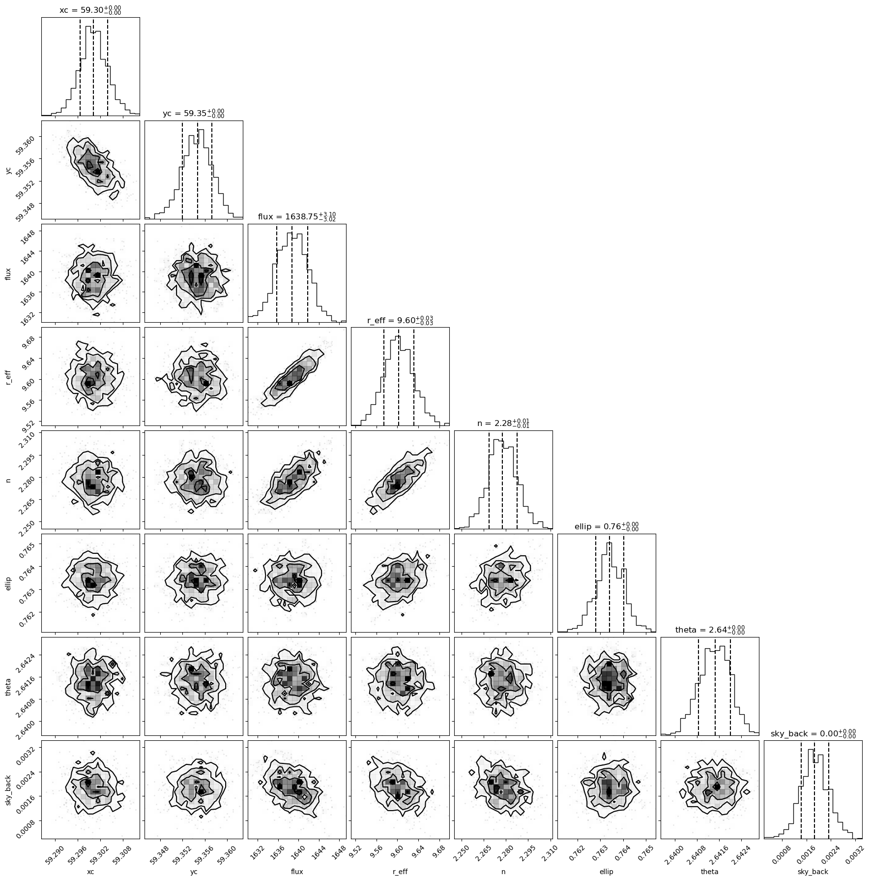
The default summary output for for the fit designates the different sources with the format _X where X is the source number. To single out any particular source, we provide a function parse_multi_results(), which allows you to specify one source at a time:

[9]:

source_res = parse_multi_results(res_mp,2) #extract source with ID 2, the large central galaxy
source_res.corner()
source_res.summary()

arviz - WARNING - Shape validation failed: input_shape: (1, 1000), minimum_shape: (chains=2, draws=4)

[9]:

	mean	sd	hdi_3%	hdi_97%	mcse_mean	mcse_sd	ess_bulk	ess_tail	r_hat
xc	59.300	0.004	59.293	59.307	0.000	0.000	918.0	943.0	NaN
yc	59.355	0.003	59.349	59.360	0.000	0.000	1166.0	900.0	NaN
flux	1638.745	3.066	1632.576	1643.946	0.103	0.073	894.0	1026.0	NaN
r_eff	9.603	0.029	9.546	9.653	0.001	0.001	938.0	959.0	NaN
n	2.278	0.010	2.259	2.297	0.000	0.000	966.0	857.0	NaN
ellip	0.763	0.001	0.762	0.764	0.000	0.000	922.0	841.0	NaN
theta	2.641	0.001	2.640	2.642	0.000	0.000	986.0	937.0	NaN
sky_back	0.002	0.000	0.001	0.003	0.000	0.000	752.0	868.0	NaN

If we now go to extract the chains, we can see that the idata property is only for this source:

[10]:

source_res.idata

To return the full dataset to the idata property, you can re-run the parser setting a source index of -1:

[11]:

source_res = parse_multi_results(source_res,-1) # put everything back

[12]:

source_res.idata