Bulge Disk Decomposition (and other “multi-profile” fits)

In this guide, we’ll briefly show the functionality for fitting multi-component profiles. Here, we will use a new sersic_exp profile, in which a sersic profile is fit to the inner portion of a galaxy, while the outer part is fit with the sersic index fixed to 1. An additional degree of flexibility can be added using doublesersic, in which the n for both profiles can vary.

import jax.numpy as jnp
import numpy as np


# Load up one of the canonical example galaxies
def load_data(n):
    im = np.load(f"examp_gals/gal{n}_im.npy")
    mask = np.load(f"examp_gals/gal{n}_mask.npy")
    sig = np.load(f"examp_gals/gal{n}_sig.npy")
    psf = np.load(f"examp_gals/gal{n}_psf.npy")
    return im, mask, sig, psf


im, mask, sig, psf = load_data(2)

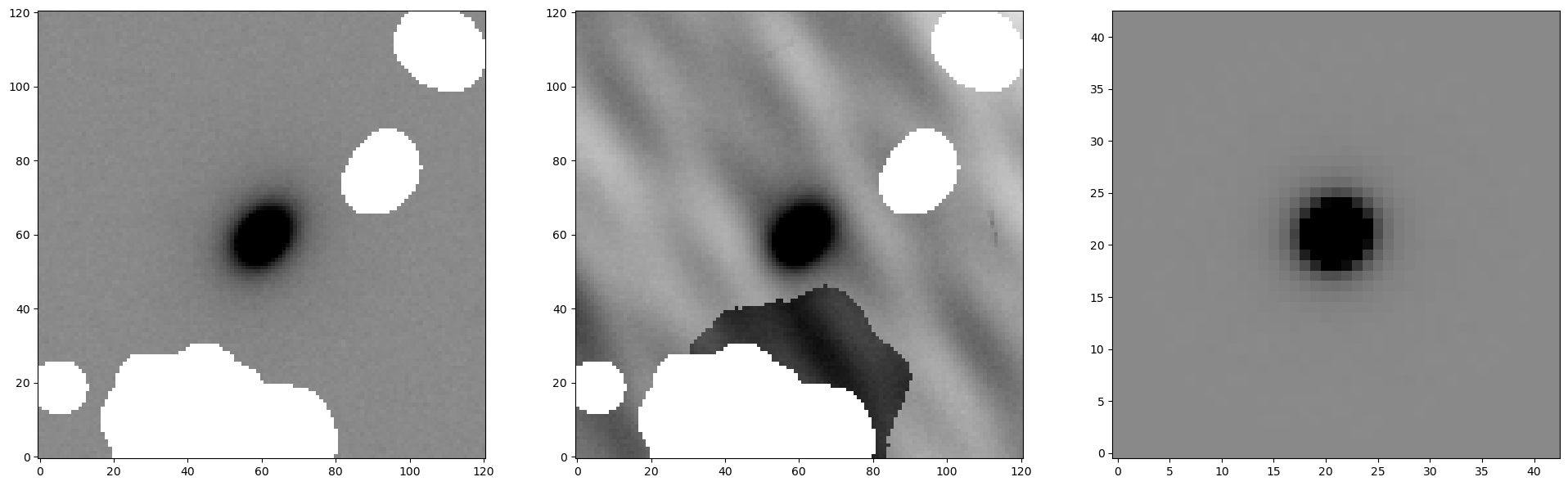
from pysersic.results import plot_image

fig, ax = plot_image(im, mask, sig, psf)

/Users/ipasha/miniforge3/envs/pysersic-14/lib/python3.11/site-packages/tqdm/auto.py:21: TqdmWarning: IProgress not found. Please update jupyter and ipywidgets. See https://ipywidgets.readthedocs.io/en/stable/user_install.html
  from .autonotebook import tqdm as notebook_tqdm

Setting up the new Prior

We have added an explict sersic_exp profile type to the list of supported options. This is similar to the doublesersic, but uses the render_exp to explicitly remove priors around the secondary “n”. One can now fit a galaxy using the same autoprior function used in the docs:

from pysersic.priors import autoprior

prior = autoprior(image=im, profile_type="sersic_exp", mask=mask, sky_type="none")

prior

Prior for a sersic_exp source:
------------------------------
flux ---  Normal w/ mu = 3689.19, sigma = 121.48
xc ---  Normal w/ mu = 60.39, sigma = 1.00
yc ---  Normal w/ mu = 59.29, sigma = 1.00
f_1 ---  Uniform between: 0.00 -> 1.00
theta ---  Uniform between: 0.00 -> 6.28
r_eff_1 ---  Truncated Normal w/ mu = 4.10, sigma = 2.03, between: 0.50 -> inf
r_eff_2 ---  Truncated Normal w/ mu = 9.23, sigma = 3.04, between: 0.50 -> inf
ellip_1 ---  Uniform between: 0.00 -> 0.90
ellip_2 ---  Uniform between: 0.00 -> 0.90
n ---  Truncated Normal w/ mu = 4.00, sigma = 1.00, between: 0.65 -> 8.00
sky type - None

In brief, the formulation for this kind of fit includes

• f_1, the fraction of total flux contained within the inner (sersic) component. The fraction in the second (exponential) component is by definition flux-f_1.

• theta, which is defined to be the same for both components at present

• r_eff_1 and r_eff_2, the two effective radii of the two components. At present, autoprior simply sets the inner profile to be the measured r_eff from a simple call to photutils data_properties divided by 1.5, and the other one to be the same times 1.5. (One can always override these). r_eff_1 should be smaller than r_eff_2.

• ellip_1 and ellip_2 are treated fully independently.

• x_c and y_c for the two models are constrained to be the precise same location.

Fitting

We can now proceed with fitting in the normal way:

from pysersic import FitSingle
from pysersic.loss import student_t_loss

fitter = FitSingle(
    data=im, rms=sig, mask=mask, psf=psf, prior=prior, loss_func=student_t_loss
)

from jax.random import (
    PRNGKey,  # Need to use a seed to start jax's random number generation
)

map_params = fitter.find_MAP(rkey=PRNGKey(1000))

 31%|███▏      | 6295/20000 [00:16<00:35, 387.20it/s, Round = 0,step_size = 5.0e-02 loss: -1.592e+04]
  1%|▏         | 252/20000 [00:00<00:50, 388.84it/s, Round = 1,step_size = 5.0e-03 loss: -1.592e+04]
  1%|▏         | 251/20000 [00:00<00:51, 387.23it/s, Round = 2,step_size = 5.0e-04 loss: -1.592e+04]

from pysersic.results import plot_residual

fig, ax = plot_residual(im, map_params["model"], mask=mask, vmin=-1, vmax=1)

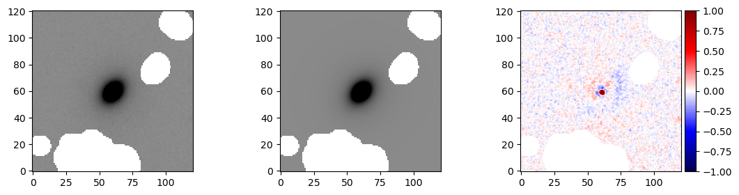
As before, map_params is a simple dictionary with some parameters and one model instance corresponding to those parameters.

map_params

{'flux': Array(3731.5237, dtype=float32),
 'xc': Array(60.43279, dtype=float32),
 'yc': Array(59.26297, dtype=float32),
 'f_1': Array(0.75661, dtype=float32),
 'theta': Array(2.43743, dtype=float32),
 'r_eff_1': Array(4.32471, dtype=float32),
 'r_eff_2': Array(19.086239, dtype=float32),
 'ellip_1': Array(0.35005, dtype=float32),
 'ellip_2': Array(0.00014, dtype=float32),
 'n': Array(2.3921099, dtype=float32),
 'model': array([[0.00290311, 0.00291601, 0.00294391, ..., 0.00273432, 0.00272112,
         0.00270705],
        [0.00292037, 0.00294186, 0.00296349, ..., 0.00275073, 0.00272958,
         0.00272279],
        [0.00295186, 0.00296701, 0.00299746, ..., 0.00276646, 0.00275226,
         0.00273767],
        ...,
        [0.00271004, 0.00271845, 0.00272568, ..., 0.00298243, 0.00294799,
         0.00292868],
        [0.0027047 , 0.0027052 , 0.00272018, ..., 0.00295745, 0.00293191,
         0.00290587],
        [0.0026981 , 0.00270633, 0.0027137 , ..., 0.00294722, 0.00291496,
         0.00289751]], dtype=float32)}

We can also run our methods to estimate or sample the posterior:

res = fitter.estimate_posterior(rkey=PRNGKey(1001), method="laplace")

  5%|▌         | 1084/20000 [00:03<00:53, 352.16it/s, Round = 0,step_size = 5.0e-02 loss: -1.594e+04]
  1%|▏         | 295/20000 [00:00<00:49, 397.46it/s, Round = 1,step_size = 5.0e-03 loss: -1.594e+04]
  2%|▏         | 354/20000 [00:00<00:50, 388.89it/s, Round = 2,step_size = 5.0e-04 loss: -1.594e+04]

summary = fitter.svi_results.summary()

arviz - WARNING - Shape validation failed: input_shape: (1, 1000), minimum_shape: (chains=2, draws=4)

summary

	mean	sd	hdi_3%	hdi_97%	mcse_mean	mcse_sd	ess_bulk	ess_tail	r_hat
ellip_1	0.221	0.004	0.212	0.228	0.000	0.000	881.0	790.0	NaN
ellip_2	0.598	0.008	0.581	0.612	0.000	0.000	941.0	850.0	NaN
f_1	0.868	0.004	0.861	0.875	0.000	0.000	978.0	908.0	NaN
flux	3996.181	17.292	3965.582	4029.488	0.545	0.385	1010.0	1023.0	NaN
n	4.665	0.077	4.528	4.804	0.002	0.002	971.0	912.0	NaN
r_eff_1	7.503	0.090	7.313	7.657	0.003	0.002	1094.0	1070.0	NaN
r_eff_2	5.047	0.068	4.928	5.185	0.002	0.001	1110.0	973.0	NaN
theta	2.439	0.003	2.434	2.443	0.000	0.000	984.0	1026.0	NaN
xc	60.438	0.003	60.433	60.443	0.000	0.000	992.0	969.0	NaN
yc	59.259	0.003	59.254	59.264	0.000	0.000	974.0	756.0	NaN

We can easily visualize the “mean model” from this SVI run by grabbing the parameter names and mean values:

dict = {}
for a, b in zip(summary.index, summary["mean"]):
    dict[a] = b

dict

{'ellip_1': 0.221,
 'ellip_2': 0.598,
 'f_1': 0.868,
 'flux': 3996.181,
 'n': 4.665,
 'r_eff_1': 7.503,
 'r_eff_2': 5.047,
 'theta': 2.439,
 'xc': 60.438,
 'yc': 59.259}

And passing them to one of our renderers, remembering to set our new profile type:

from pysersic.rendering import HybridRenderer

bf_model = HybridRenderer(im.shape, jnp.array(psf.astype(np.float32))).render_source(
    dict, profile_type="sersic_exp"
)

from pysersic.results import plot_residual

fig, ax = plot_residual(im, bf_model, mask=mask, vmin=-1, vmax=1)

Further Steps

If you are interested in getting deeper into multi-component fitting, check out the “manual priors” tutorial. There you can see how to set all the priors of a sersic_exp or doublesersic profile to more specific bounds, if the autoprior is insufficient for your needs. If you have strong reasons to actually change the fitting nature (e.g., offset components spatially, or different thetas for the two components), please reach out and let us know.