Pysersic Walkthrough: Fitting a single source

In this tutorial we’ll walk through how to set up and fit a galaxy using pysersic.

Loading the data

We’ll be using three galaxies imaged by HSC for this example. The 4 needed inputs to perform a fit are

im: the image itself
mask: a mask indicating pixels which should not be included in the fit
sig: a map of pixel uncertainties
psf: a map of the PSF (for now, only one psf can be used).

[1]:

import numpy as np
def load_data(n):
    im = np.load(f'examp_gals/gal{n}_im.npy')
    mask = np.load(f'examp_gals/gal{n}_mask.npy')
    sig = np.load(f'examp_gals/gal{n}_sig.npy')
    psf = np.load(f'examp_gals/gal{n}_psf.npy')
    return im,mask,sig,psf

im,mask,sig,psf = load_data(2)

Let’s visualize our galaxy, just to see what we’re working with. You can do this any way you like. A convenience function is provided:

[2]:

from pysersic.results import plot_image

fig, ax = plot_image(im,mask,sig,psf)

We can also check that our inputs — the image, mask, rms map, and psf — conform to the necessary shapes and sizes for a pysersic run.

In particular, our psf map must be smaller than the input data image, and the data, rms, and mask (if provided) must have the same shape.

The pysersic code will automatically check your input data for goodness when it runs, but if you would like to check before attempting to run pysersic, you can do so via the following:

[3]:

from pysersic import check_input_data

check_input_data(data=im,rms=sig,psf=psf,mask=mask)

[3]:

True

This function will return True if all checks pass, otherwise it will raise a warning or exception if something is amiss.

Fitting

Now that we have our galaxy to fit, we can get set up with pysersic.

Because we are fitting a single source, we’ll want to initialize a pysersic.FitSingle object. For a field with multiple object, we would use pysersic.FitMulti.

Additionally, we will need to set up a pysersic.PysersicSourcePrior object to handle the priors for the fit. (Again, using Source as we have a single galaxy to fit).

The Source Prior takes two initial arguments, the profile type, whose options at current are

sersic
pointsource
exponential
devaucoleurs

and two compound profiles

doublesersic (2 sersic profiles with a shared center and PA)
sersic_pointsource (shared center)

and the sky_type, which indicates whether to fit the sky background, either with

none (no fitting)
flat (constant offset), or
tilted-plane

At this point, we would need to write down priors for all of the fit parameters of a Sersic. However, there is an autoprior function that measures the observed properties of the source using the photutils package to help us with this:

[4]:

from pysersic.priors import autoprior

prior  = autoprior(image = im, profile_type = 'sersic', mask=mask, sky_type = 'none')

The generate_prior() function has a built-in choices about the prior functions to use for each sersic parameter based off of the observed properties. These seem to work decently well in a lot of cases we tested but may not work for you! We can also specify if we want to add a sky model, here we will not. To see more about customizing priors, see the manual-priors example notebook or the documentation. For now we will print our prior:

[5]:

prior

[5]:

Prior for a sersic source:
--------------------------
flux ---  Normal w/ mu = 3689.19, sigma = 121.48
xc ---  Normal w/ mu = 60.39, sigma = 1.00
yc ---  Normal w/ mu = 59.29, sigma = 1.00
r_eff ---  Truncated Normal w/ mu = 6.16, sigma = 4.96, between: 0.50 -> inf
ellip ---  Uniform between: 0.00 -> 0.90
theta ---  Uniform between: 0.00 -> 6.28
n ---  Uniform between: 0.65 -> 8.00
sky type - None

As we can see, this function used properties of the input image to make reasonable priors for the fit parameters. For now, let’s continue, and in another example, we’ll set some priors manually.

Armed with our prior object, we can set up our FitSingle fitter. At this stage, we need to choose a loss_func(), which is used to evaluate the models to the data. For this example, we’ll import the student_t_loss() from the utils.loss submodule. This is a decent starting place as it is less sensitive to outliers than a gaussian (i.e. \(\chi^2\)) loss.

[6]:

from pysersic import FitSingle
from pysersic.loss import student_t_loss

fitter = FitSingle(data=im,rms=sig,mask=mask,psf=psf,prior=prior,loss_func=student_t_loss)

There are a set of currently loss functions already coded up in loss py, some of which include:

Cash loss using Poisson Statistics(Cash 1979)
Gaussian loss with a free systematic scatter parameter
Gaussian mixture loss with representing an outlier distribution

See the page on Loss Functions to learn more about these choices.

With a fitter object created, we are now free to carry out a fit.

MAP Parameters

Before we jump all the way into sampling, it’s worth noting that we can also retrieve a prediction for the best fit model very quickly, using SVI (stochastic variational inference).

The simplest, barebones way to do this is to run the fitter.find_MAP() method. This will produce a point-estimate of the parameters with no attempt to estimate the posterior distribution (i.e., the closest thing to running GALFIT). Unlike the rest of the methods we’ll show below, this does not produce a fancy PySersicResult object; it simply returns a dictionary with the values:

[7]:

from jax.random import PRNGKey # Need to use a seed to start jax's random number generation
map_params = fitter.find_MAP(rkey = PRNGKey(1000))

  2%|▏         | 423/20000 [00:00<00:41, 468.62it/s, Round = 0,step_size = 5.0e-02 loss: -1.537e+04]
  1%|▏         | 252/20000 [00:00<00:41, 478.15it/s, Round = 1,step_size = 5.0e-03 loss: -1.537e+04]
  2%|▏         | 383/20000 [00:00<00:41, 476.45it/s, Round = 2,step_size = 5.0e-04 loss: -1.537e+04]

[8]:

map_params

[8]:

{'flux': Array(3756.919, dtype=float32),
 'xc': Array(60.43696, dtype=float32),
 'yc': Array(59.25185, dtype=float32),
 'r_eff': Array(6.25733, dtype=float32),
 'ellip': Array(0.31224, dtype=float32),
 'theta': Array(4.01482, dtype=float32),
 'n': Array(3.64185, dtype=float32),
 'model': array([[0.00421399, 0.00437032, 0.0045427 , ..., 0.0009528 , 0.00091871,
         0.00087596],
        [0.0043357 , 0.004512  , 0.00468226, ..., 0.00099302, 0.00094683,
         0.00091467],
        [0.00447063, 0.00464482, 0.00483559, ..., 0.00102401, 0.00098818,
         0.00094428],
        ...,
        [0.00086259, 0.00090328, 0.00093473, ..., 0.00477184, 0.00458993,
         0.00442436],
        [0.00083635, 0.00086465, 0.00090682, ..., 0.00461365, 0.0044527 ,
         0.00428449],
        [0.00080035, 0.00083954, 0.00086964, ..., 0.00447006, 0.00430648,
         0.00415841]], dtype=float32)}

We can then use the plot_residual function to quickly compare model to the data:

[9]:

from pysersic.results import plot_residual
fig, ax = plot_residual(im,map_params['model'],mask=mask,vmin=-1,vmax=1)

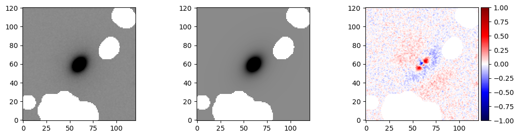
Without compilation (i.e., after being run once), running this took ~3 seconds on the laptop on which this notebook was run (on CPU). Including compilation, it is closer to ~5s.

Posterior Estimation

Taking one step up from simply retrieving the MAP, we can make an estimate of the posterior around the MAP using one of several available methods.

At present, these are laplace, in which the MAP is found, then the posterior is assumed to be a gaussian around it, and svi-flow, in which a normalizing flow is trained to estimate the posterior and is sampled from directly.

Both methods are relatively fast, with laplace taking 8-10 seconds and svi-flow taking around 45 seconds.

[10]:

res = fitter.estimate_posterior(rkey = PRNGKey(1001), method='laplace')

  2%|▏         | 387/20000 [00:00<00:39, 498.77it/s, Round = 0,step_size = 5.0e-02 loss: -1.537e+04]
  2%|▏         | 321/20000 [00:00<00:39, 502.04it/s, Round = 1,step_size = 5.0e-03 loss: -1.537e+04]
  3%|▎         | 545/20000 [00:01<00:38, 502.42it/s, Round = 2,step_size = 5.0e-04 loss: -1.537e+04]

[11]:

res2 = fitter.estimate_posterior(rkey = PRNGKey(1002),method='svi-flow')

  8%|▊         | 1624/20000 [00:16<03:10, 96.57it/s, Round = 0,step_size = 5.0e-02 loss: -1.534e+04]
  4%|▍         | 850/20000 [00:08<03:22, 94.60it/s, Round = 1,step_size = 5.0e-03 loss: -1.534e+04]
  3%|▎         | 548/20000 [00:05<03:24, 95.04it/s, Round = 2,step_size = 5.0e-04 loss: -1.534e+04]

As a note, these fit methods return the results object, but we can access it anytime by calling the fitter.svi_results attribute. But a given fitter can only have one svi_results and one sampling_results at a time, hence the use of res2 above to extract it separately

For any run, we can use the .summary() method of the fitter.svi_results to see a dataframe output.

[12]:

fitter.svi_results.summary()

arviz - WARNING - Shape validation failed: input_shape: (1, 1000), minimum_shape: (chains=2, draws=4)

[12]:

	mean	sd	hdi_3%	hdi_97%	mcse_mean	mcse_sd	ess_bulk	ess_tail	r_hat
ellip	0.312	0.002	0.308	0.315	0.000	0.000	873.0	662.0	NaN
flux	3756.890	8.683	3739.934	3772.259	0.283	0.200	939.0	888.0	NaN
n	3.643	0.023	3.600	3.682	0.001	0.001	943.0	932.0	NaN
r_eff	6.253	0.027	6.200	6.299	0.001	0.001	927.0	834.0	NaN
theta	0.873	0.003	0.867	0.879	0.000	0.000	975.0	979.0	NaN
xc	60.437	0.003	60.430	60.442	0.000	0.000	999.0	950.0	NaN
yc	59.252	0.003	59.245	59.258	0.000	0.000	1016.0	980.0	NaN

Sampling

Let’s now try to sample. Here, we use the efficiency of No U-turn sampling plus the jit-compiled nature of the codebase to generate e.g., 4000 samples relatively quickly (<1 min per chain).

We can run the fitter.sample() method with no arguments, which will default to 2000 samples in 2 chains. But sample() will take any **kwargs to be passed to the mcmc.NUTS() sampler under the hood. The fitter.sample() method returns a new instance of a PySersicResults object, but will also store that new result in an attribute fitter.sampling_results, so we don’t explicitly have to define a name here:

[13]:

fitter.sample(rkey = PRNGKey(1003))

/Users/timothymiller/Documents/research/packages/pysersic/pysersic/pysersic/pysersic.py:140: UserWarning: There are not enough devices to run parallel chains: expected 2 but got 1. Chains will be drawn sequentially. If you are running MCMC in CPU, consider using `numpyro.set_host_device_count(2)` at the beginning of your program. You can double-check how many devices are available in your system using `jax.local_device_count()`.
  sampler =infer.MCMC(infer.NUTS(model,init_strategy=init_strategy, **sampler_kwargs),num_chains=num_chains, num_samples=num_samples, num_warmup=num_warmup,  **mcmc_kwargs)
sample: 100%|██████████| 2000/2000 [00:56<00:00, 35.65it/s, 11 steps of size 2.34e-01. acc. prob=0.93]
sample: 100%|██████████| 2000/2000 [00:47<00:00, 42.20it/s, 7 steps of size 2.52e-01. acc. prob=0.91]

[13]:

PySersicResults object for pysersic fit of type: sampling

If we want to see the reuslts, we can retrieve an arviz summary table the same way as before, but this time retrieving the sampling results:

[14]:

sampling_res = fitter.sampling_results
sampling_res.summary()

[14]:

	mean	sd	hdi_3%	hdi_97%	mcse_mean	mcse_sd	ess_bulk	ess_tail	r_hat
ellip	0.312	0.002	0.309	0.316	0.000	0.000	1621.0	1300.0	1.0
flux	3757.306	8.437	3742.038	3772.960	0.310	0.219	739.0	1009.0	1.0
n	3.643	0.023	3.598	3.683	0.001	0.001	710.0	1151.0	1.0
r_eff	6.257	0.027	6.211	6.309	0.001	0.001	809.0	1096.0	1.0
theta	0.873	0.003	0.868	0.880	0.000	0.000	2757.0	1412.0	1.0
xc	60.437	0.003	60.431	60.443	0.000	0.000	2025.0	1339.0	1.0
yc	59.252	0.004	59.245	59.259	0.000	0.000	1722.0	1124.0	1.0

Other Diagnostics and Visualizations

Below we cover a few diagnostics we can look at.

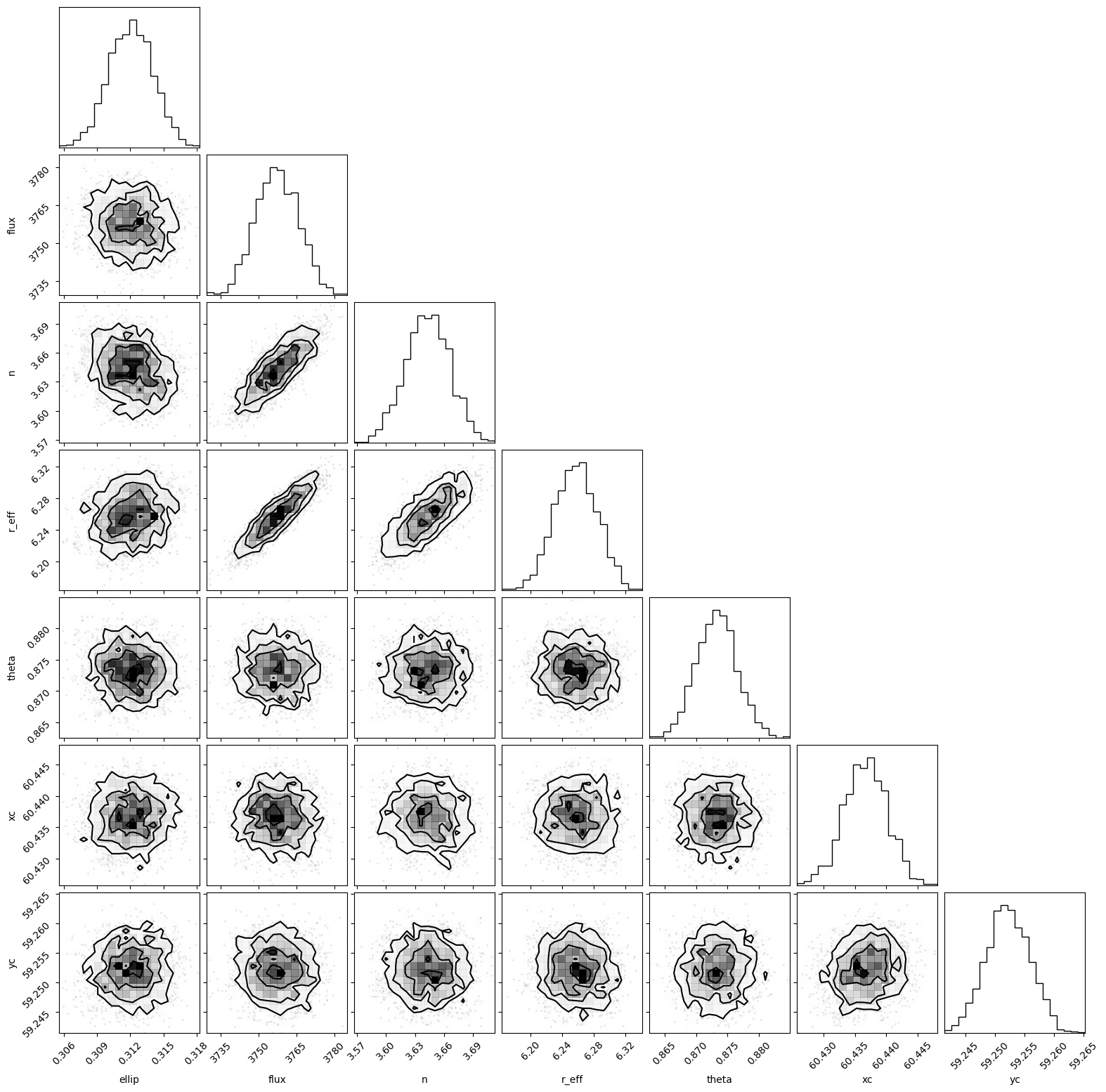
We can, for example, create corner plots for either the SVI results or sampling results:

[15]:

fig = fitter.svi_results.corner()

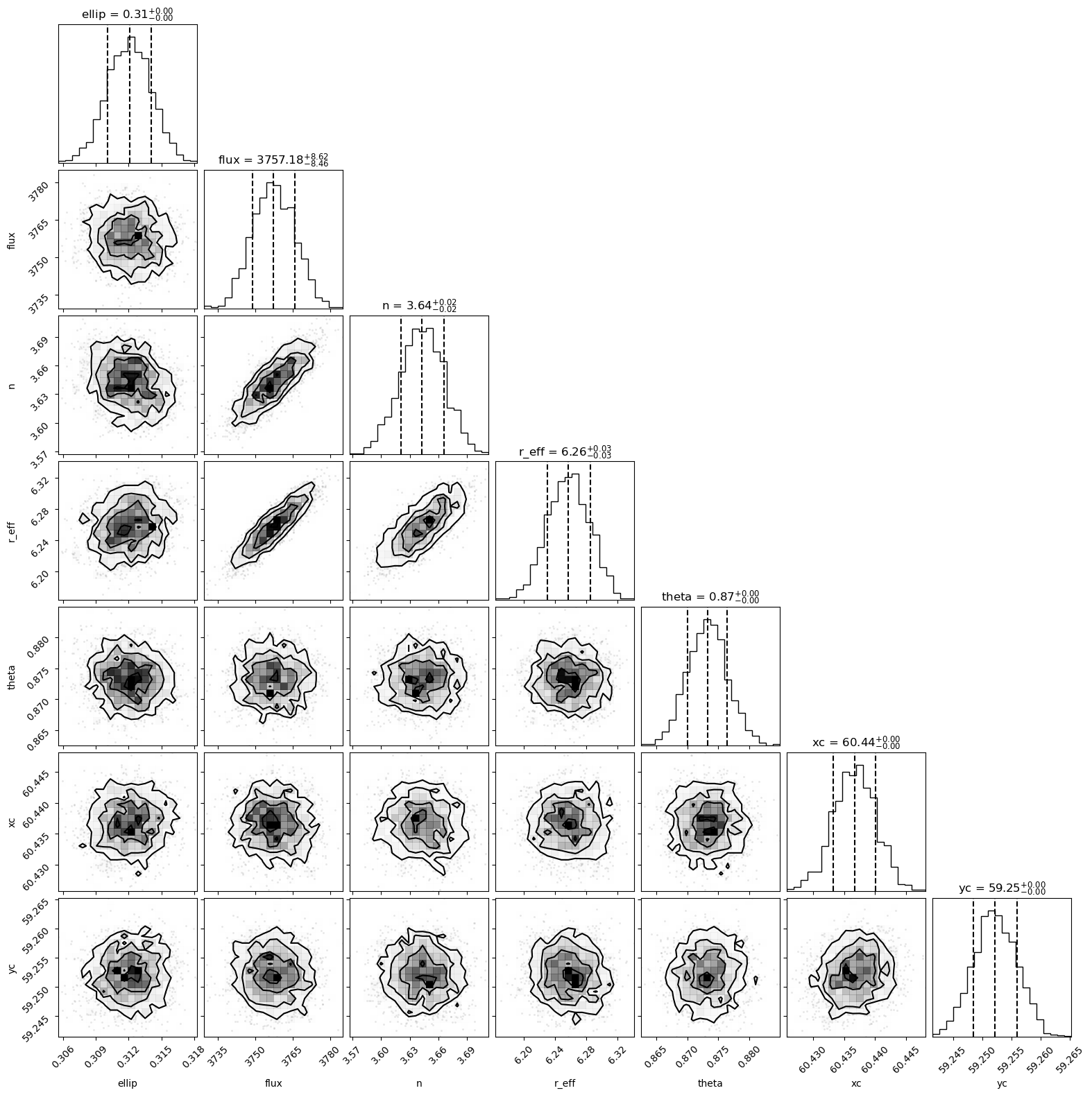
[16]:

fig = fitter.sampling_results.corner()

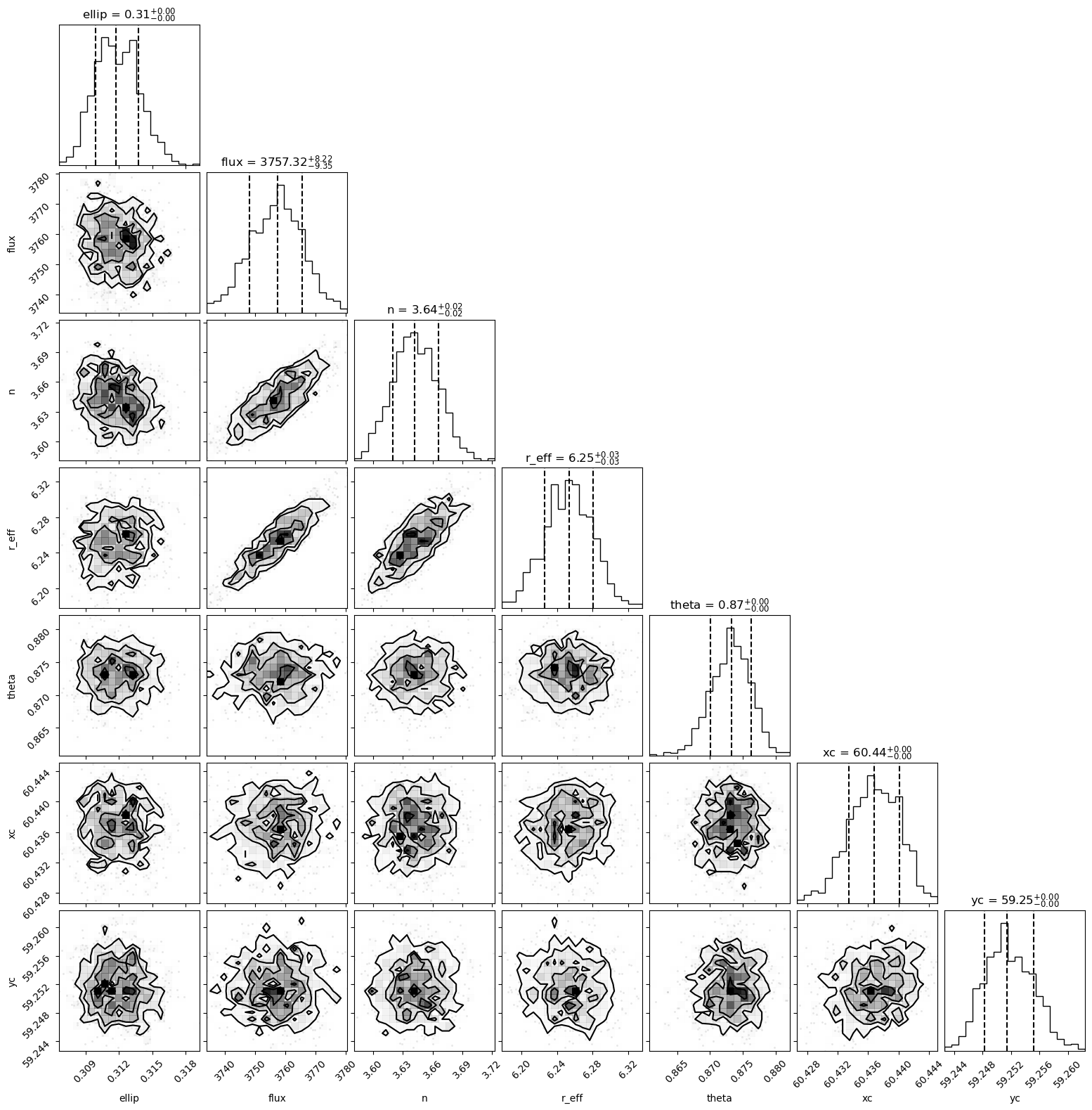
It is relatively easy with the corner.py package to overplot both on each other to see how similar they are:

[17]:

import corner
fig = fitter.sampling_results.corner(color='C0')
fig = corner.corner(fitter.svi_results.idata,quantiles=[.16,.5,.84],color='C1',fig=fig)

If we want to retrieve a table with arbitrary quantiles for a fit, we can use the retrieve_param_quantiles() function. This will return either a dictionary (if return_dataframe=False) or a data frame, with the requested quantiles as columns and the parameters as rows.

[18]:

fitter.svi_results.retrieve_param_quantiles(return_dataframe=True)

[18]:

	0.16	0.50	0.84
ellip	0.309881	0.311757	0.313792
flux	3747.969883	3757.317017	3765.539111
n	3.620020	3.642152	3.666159
r_eff	6.226340	6.253471	6.280443
theta	0.870076	0.873307	0.876258
xc	60.433497	60.436821	60.440117
yc	59.248287	59.251436	59.255228

[19]:

fitter.svi_results.retrieve_param_quantiles(return_dataframe=False)

[19]:

{'ellip': [0.3098809278011322, 0.31175675988197327, 0.3137915074825287],
 'flux': [3747.9698828125, 3757.3170166015625, 3765.539111328125],
 'n': [3.6200195217132567, 3.6421520709991455, 3.6661585426330565],
 'r_eff': [6.226339988708496, 6.2534708976745605, 6.280443286895752],
 'theta': [0.8700764274597168, 0.8733072280883789, 0.8762576866149903],
 'xc': [60.43349655151367, 60.43682098388672, 60.44011749267578],
 'yc': [59.24828659057617, 59.25143623352051, 59.255227966308595]}

As a note, the default returned quantiles are [0.16, 0.5, 0.84] but you can specify any quantiles you wish to the method. The same syntax above will work with the fitter.sampling_results as well — they are the same underlying class.

[20]:

fitter.sampling_results.retrieve_param_quantiles(return_dataframe=True)

[20]:

	0.16	0.50	0.84
ellip	0.310048	0.312118	0.314096
flux	3748.721631	3757.179688	3765.799922
n	3.620633	3.642768	3.665765
r_eff	6.230554	6.257283	6.285270
theta	0.870078	0.873290	0.876375
xc	60.433291	60.436684	60.440053
yc	59.248428	59.252138	59.255979

We can also print out a latex-ready table (using the AAStex deluxetable), if we would so like (the data portion of the table is easily copy-able to other formats).

[21]:

fitter.sampling_results.latex_table()

\begin{deluxetable}{lr}[b]
\tablehead{
\colhead{Parameter} & \colhead{\hspace{4.5cm}Value\hspace{.5cm}}}
\caption{Best Fit Parameters for Pysersic Fit}
\startdata
ellip & 0.312_{-0.002}^{+0.002} \\
flux & 3757.180_{-8.458}^{+8.620} \\
n & 3.643_{-0.022}^{+0.023} \\
r_{\rm eff} & 6.257_{-0.027}^{+0.028} \\
\theta & 0.873_{-0.003}^{+0.003} \\
xc & 60.437_{-0.003}^{+0.003} \\
yc & 59.252_{-0.004}^{+0.004} \\
\enddata
\end{deluxetable}

We can also use any callable func on any parameter via the following:

[22]:

ellip_std = fitter.sampling_results.compute_statistic(parameter='ellip',func=np.std)
ellip_std

[22]:

array(0.00201616, dtype=float32)

Finally, if we just want to yank the chains and start doing our own thing with them, note that the results object has an attribute .idata which is an arviz.InferenceData object, so it can be slotted into many analyses. We do have a handy function for extracting the chains for each parameter, though:

[23]:

sampling_chain = fitter.svi_results.get_chains()
sampling_chain['n']

There are many more things we can do in terms of carrying out statistics on our outputs – but since arviz has its own, well-vetted system for that, we trust that you can grab the arviz inference data objects (fitter.svi_results.idata and fitter.sampling_results.idata) and run with them as needed, inserting them into other analyses.

Saving the fit to a file

Lastly, we may want to save the parameters of our fit (info, chains, models, data) to a file. This can be done with the results.save_results() method:

As we can see, the information needed to reconsitute the models and fit parameters are all stored in this file. The 'input_data' dictionary in the tree contains a copy of the data that was fit. We can see which loss function and renderer was used. We can also access our prior printout:

[24]:

fitter.sampling_results.save_result('example_fit.asdf')

We can (presumably at a later time) then load our asdf file and view what it contains:

[25]:

import asdf
af = asdf.open('example_fit.asdf')
af.info()

root (AsdfObject)
├─asdf_library (Software)
│ ├─author (str): The ASDF Developers
│ ├─homepage (str): http://github.com/asdf-format/asdf
│ ├─name (str): asdf
│ └─version (str): 2.15.2
├─history (dict)
│ └─extensions (list) ...
├─input_data (dict)
│ ├─image (NDArrayType): shape=(121, 121), dtype=float32
│ ├─mask (NDArrayType): shape=(121, 121), dtype=bool
│ ├─psf (NDArrayType): shape=(43, 43), dtype=float32
│ └─rms (NDArrayType): shape=(121, 121), dtype=float32
├─loss_func (str): <function student_t_loss at 0x2b44dd5a0>
├─method_used (str): sampling
├─posterior (dict)
│ ├─ellip (NDArrayType): shape=(2, 1000), dtype=float32
│ ├─flux (NDArrayType): shape=(2, 1000), dtype=float32
│ ├─n (NDArrayType): shape=(2, 1000), dtype=float32
│ ├─r_eff (NDArrayType): shape=(2, 1000), dtype=float32
│ └─3 not shown
├─prior_info (str): Prior for a sersic source:
--------------------------
flux ---  Normal w (truncated)
└─rendere_type (str): <class 'pysersic.rendering.HybridRenderer'>
Some nodes not shown.

As we can see, everything we need, from the input data, to which loss function, to the prior info, and finally the posterior chains, are stored in this file. For example, to see what our priors were:

[26]:

print(af.tree['prior_info'])

Prior for a sersic source:
--------------------------
flux ---  Normal w/ mu = 3689.19, sigma = 121.48
xc ---  Normal w/ mu = 60.39, sigma = 1.00
yc ---  Normal w/ mu = 59.29, sigma = 1.00
r_eff ---  Truncated Normal w/ mu = 6.16, sigma = 4.96, between: 0.50 -> inf
ellip ---  Uniform between: 0.00 -> 0.90
theta ---  Uniform between: 0.00 -> 6.28
n ---  Uniform between: 0.65 -> 8.00
sky type - None

And finally, the posterior chains for the fits are in the 'svi_posterior' and 'sampling_posterior' dictionaries within the tree. As a result, we can quickly re-constitute a corner plot:

[27]:

import corner
fig = corner.corner(af.tree['posterior'])